Processing Streamlines and Autocorrelation from SAXS
In this post we will show streamlines created by using PCA on X-scattering images, and a derivation to get the relationship between SAXS intensity images and autocorrelation for a local state
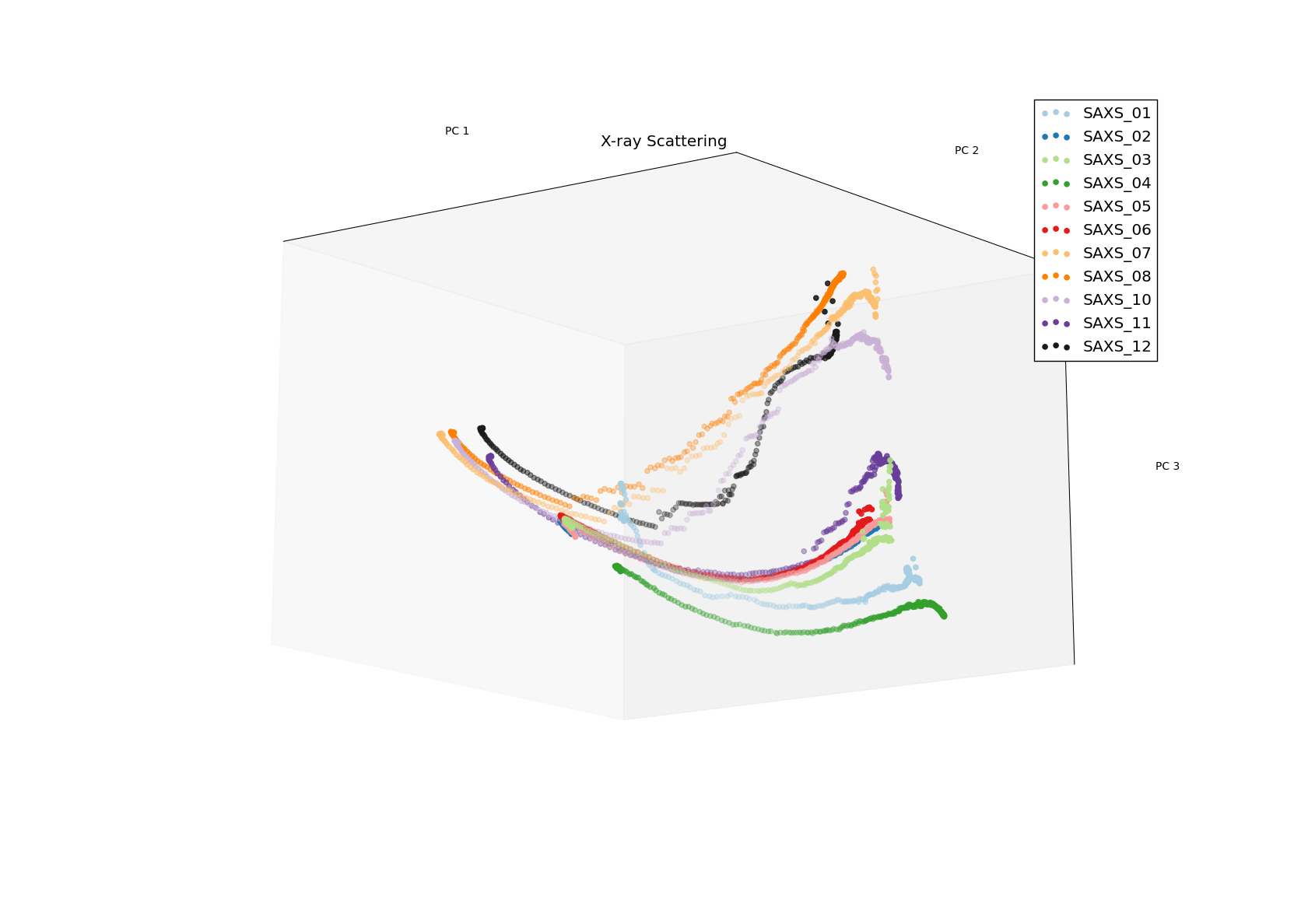
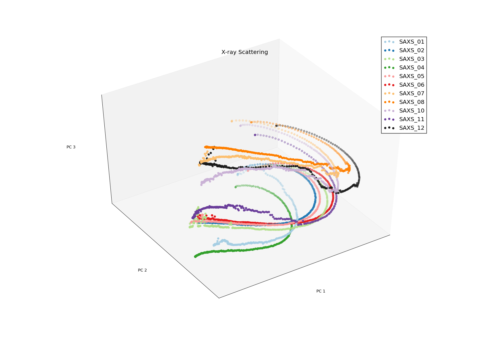
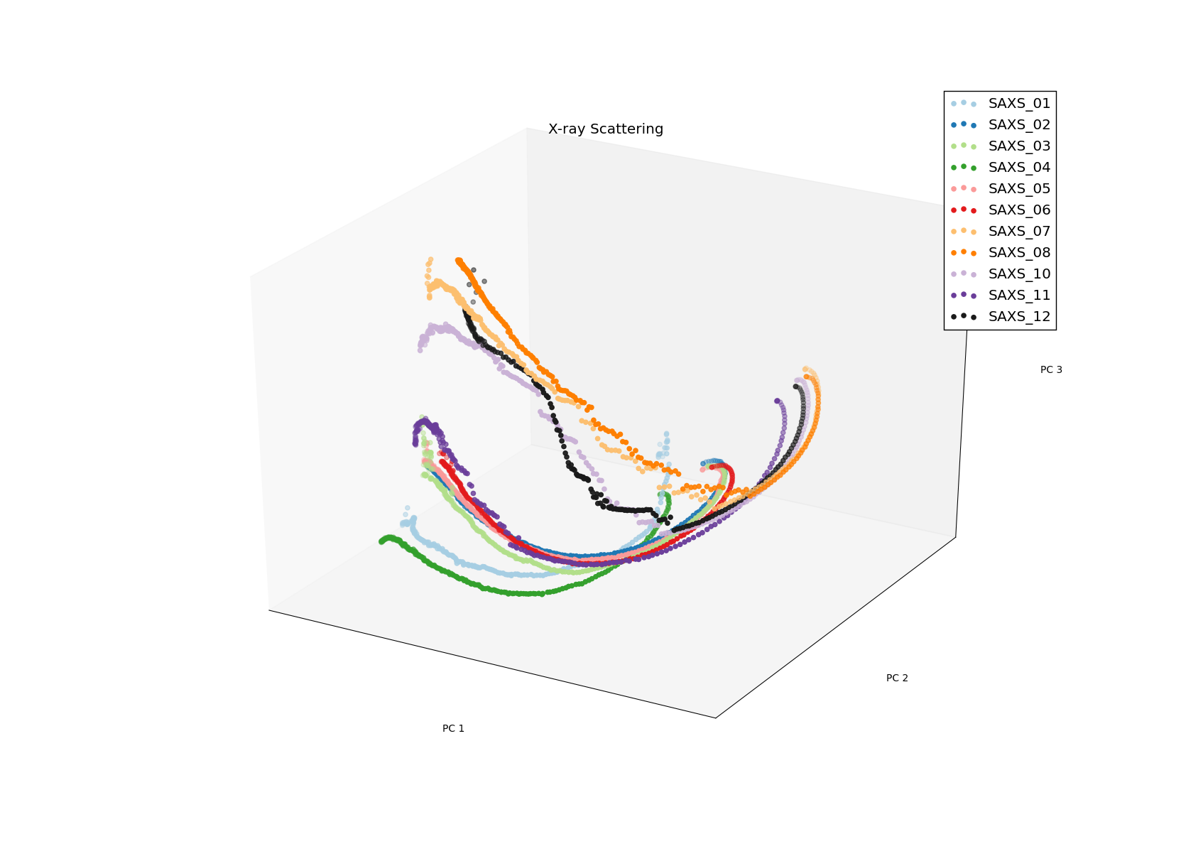
Processing Streamline from X-ray Scattering Intensity Images
The images below are three images of processing streamlines for twelve samples that an applied strain at each time step.
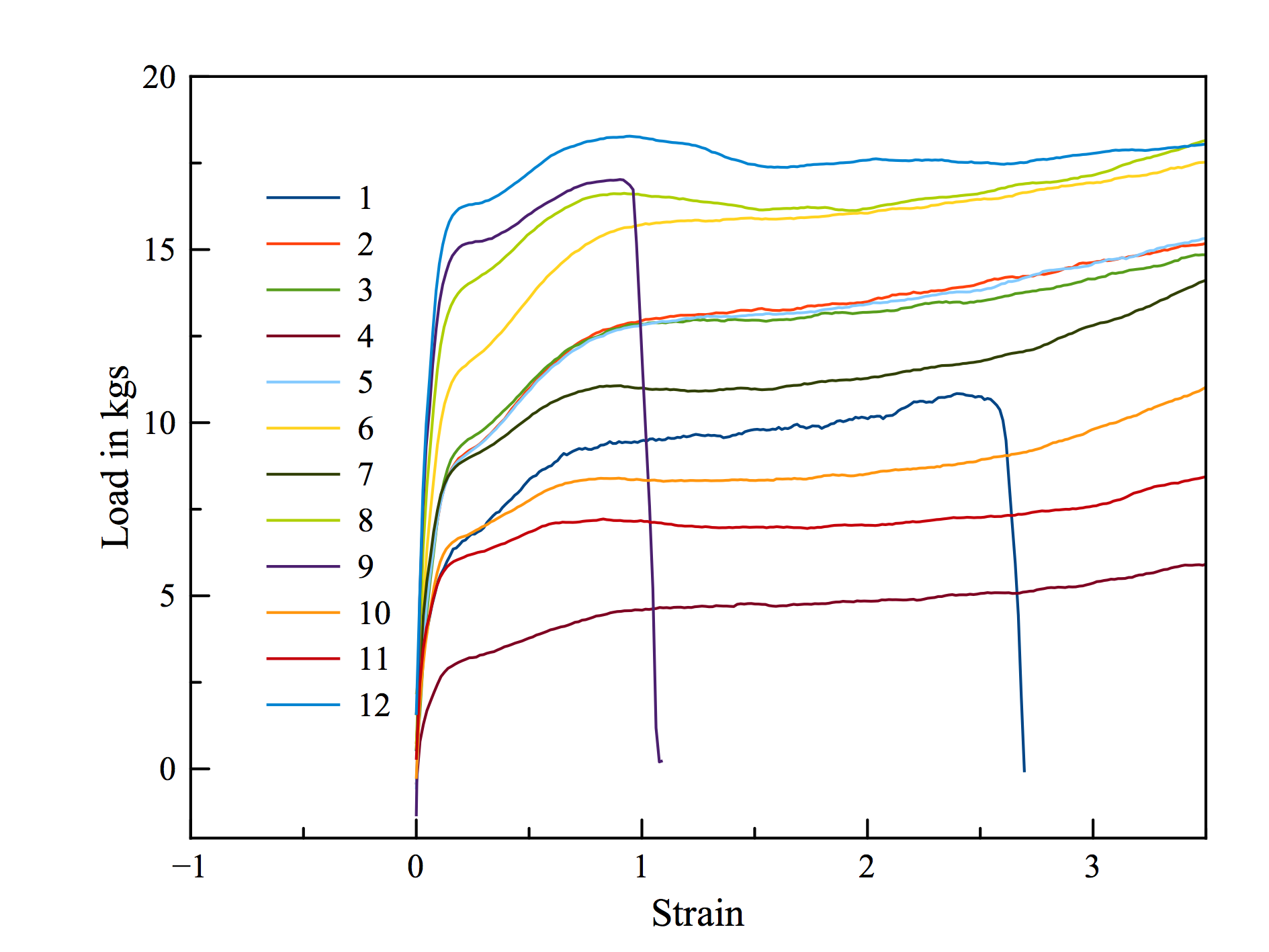
Load - Strain Behaviour for the samples explored in PCA Space
At each time step (also the strain step in this case) we have access to the % crystallinity measurements obtained independently of the SAXS data. We expect to map tthe strain and percent crystallinity to the reduced data inorder to develop predictive analytics for new microstructures.
Autocorrelation of a Local State from SAXS Data and Volume Fraction
This derivation shows how to come up with the following relationship between SAXS intensity images, volume fraction and autocorrelation of one local state for a system with only 2 local states.
\begin{eqnarray} f^{11}( \pmb x) = \frac{1}{V \eta_o^2} \int I (\pmb k) e^{-i \pmb k \pmb x} d \pmb k + V_1^2 \end{eqnarray} If we can learn how to handle the portion of the data from the beam stop, we should be able to recover the autocorrelation for the crystalline state.