Final Post
Project Definition
Description
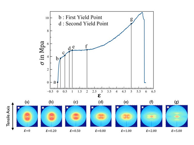
Our dataset consisted of X-ray scattering intensity images from 12 different samples of polyethylene. While each of the samples were being strain, the stress in the sample was measured and an X-scattering intensity image was taken roughly every four seconds. The twelve samples varied systematically between difference in densities, processing conditions, and thickness.
Click to see video
Dataset
The table below shows the density, thickness and processing condition for the twelve samples.
| Density (gm/cc) | Thickness (µm) | Processing Condition |
|---|---|---|
| 0.912 | 20 | A |
| 0.912 | 30 | A |
| 0.912 | 75 | A |
| 0.912 | 20 | B |
| 0.912 | 30 | B |
| 0.912 | 75 | B |
| 0.923 | 20 | A |
| 0.923 | 30 | A |
| 0.923 | 75 | A |
| 0.923 | 20 | B |
| 0.923 | 30 | B |
| 0.923 | 75 | B |
In this project we worked towards generating structure-processing linkage between the polyethylene samples and the strain applied to each sample.
Challenges
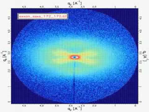
A considerable amount of time was spent trying to recover the 2-point statistics from the Small Angle X-ray Scattering (SAXS) images. Although we understood the need to take a Fourier transform of the image (a shown in this post as well as this post), we were unclear how to interpret the physical meaning of these images in real space.
Late in the semester, we were able to meet with Dr. Garmestani from the Materials Science and Engineering department at Georgia Tech. In previous research his group was able to recover pair correlation function for a 2-phase material from SAXS data. From this information, we were able to derive the relationship to get the 2-point statistics from the SAXS images.
Unfortunately because we found this relationship too late in the semester to use the 2-point statistics for the linkage, but we are interested in using the 2-point statistics to do microstructure reconstruction from the SAXS images in the future.
Collaboration
Abhiram comes from the Materials Science and Engineering department, while David comes from the Computational Science and Engineering department. Abhiram cleaned and selected the dataset for this project as well as contributed to posts and some coding. David coded most of the classes and function used for dimensionality reduction and the processing linkage. He also contributed to posts and worked out derivations.
We had several conversations with Dr. Kalidindi that were useful in determining a project direction. We also met with Dr. Garmestani to discuss the relationship between X-ray data and pair correlation functions.
Trials - Success and Failures
We spent a significant time trying to understand the physical interpretation of the Fourier transform of the SAXS images. We believe we have a good enough understanding to generate the 2-point statistics as this project continues.
Originally PCA was used on the entire X-ray scattering image to do dimensionality reduction. This turned out to be somewhat slow because of the size of the images and because of some of the data structures were initially being used in our code.
Later the dimeion_reducer class was created that would allow for flexibility in selecting a dimensionality reduction technique. This class was designed to integrate well with machine learn python package scikit-learn.

Original Scattering Image
After trying several variations on PCA, we found that kernel PCA with a linear kernel gave us the same reduced representation an order of magnitude faster than PCA. We also explored sparse PCA and found that is gave similar results to PCA and kernel PCA, but we not as fast as kernel PCA.
Because the signal strength for each image is very low, the log of every pixel was used. In order to account for the variation in X-ray scattering intensity due to sample in thickness, we divided each image by the mean intensity. Before doing PCA, we removed the areas of the images that did not contain scattering from the polyethylene.
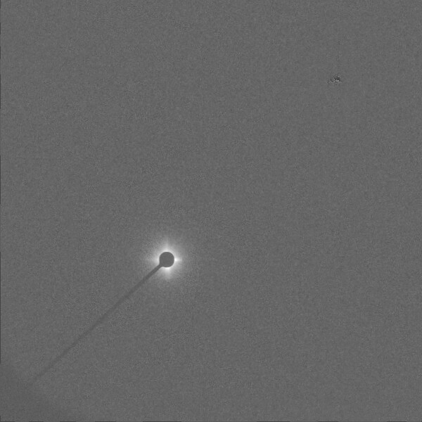
Image used in Kernel PCA
We attempted to use a completely new framework for determining a structure-processing relationship. Previously a numerical integration approach has been used to construct these linkages. In this project we used a statistical model know as transfer function model. The transfer function model can be thought of as a method to use regression for digital filter design for time varying signals.
In our case, we found that a model with the order (2, 1, 5) gave us the best result. The 2 represents the number of autoregressive terms in the model, 1 represents the number of times the time series were differenced and 5 represents the previous time steps used from an exogenous (input) series, in our case we used the measured strain values. Our model equation took the following form.
In equation above, $X_t$ is value for a given principle component over time, and $\varepsilon_t$ is the measured strain for the sample. Because the trajectories for the low density samples has different characteristics than the trajectories for the high density samples, we took on sample from each of the and fit the coefficients of our model to them. Below are a few images of the predicted processing paths compared to original data.
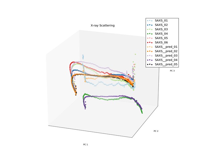
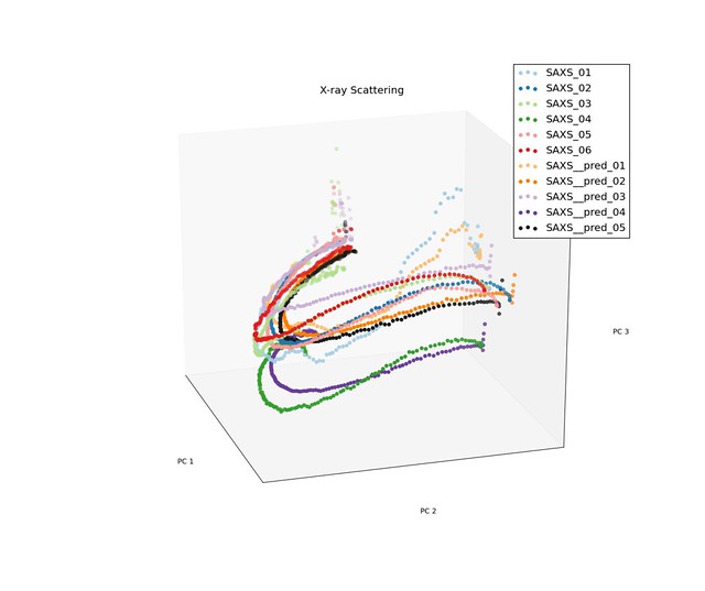
Prediction for Low Density Samples
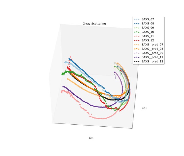
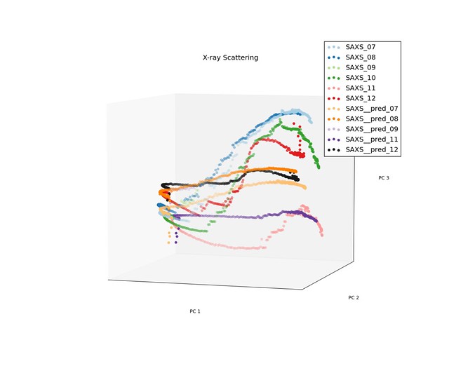
Prediction for High Density Samples
The model performed reasonable well for the low density samples, but do not preform well for the high density samples when the trajectories had discontinuities.
Overall the transfer function model did show some promise as a method to find structure processing linkages. More work will have to be done to explore improvements.
Conclusion
This project provided a great foundation for continued collaboration with this dataset. A new method to find structure processing linkages was used. In the future we hope to be able to do microstructure reconstruction as well as find a perhaps a better statistical model to predict these trajectories in the low dimensional representation.